Text classification with penalized logistic regression
This article demonstrates a modeling example using the tidymodels framework for text classification. Data are downloaded via the gutenbergr package, including 5 books written by either Emily Brontë or Charlotte Brontë. The goal is to predict the author given words in a line, that is the probability of line being written by one sister instead of another.
The cleaned books dataset contains linse as individual rows.
mirror_url <- "http://mirrors.xmission.com/gutenberg/"

books <- gutenberg_works(author %in% c("Brontë, Emily", "Brontë, Charlotte")) %>%
  gutenberg_download(meta_fields = c("title", "author"), mirror = mirror_url) %>%
  transmute(title,
            author = if_else(author == "Brontë, Emily",
                             "Emily Brontë",
                             "Charlotte Brontë") %>% factor(),
            line_index = row_number(),
            text)
books
#> # A tibble: 89,588 × 4
#>    title             author       line_index text
#>    <chr>             <fct>             <int> <chr>
#>  1 Wuthering Heights Emily Brontë          1 "Wuthering Heights"
#>  2 Wuthering Heights Emily Brontë          2 ""
#>  3 Wuthering Heights Emily Brontë          3 "by Emily Brontë"
#>  4 Wuthering Heights Emily Brontë          4 ""
#>  5 Wuthering Heights Emily Brontë          5 ""
#>  6 Wuthering Heights Emily Brontë          6 ""
#>  7 Wuthering Heights Emily Brontë          7 ""
#>  8 Wuthering Heights Emily Brontë          8 "CHAPTER I"
#>  9 Wuthering Heights Emily Brontë          9 ""
#> 10 Wuthering Heights Emily Brontë         10 ""
#> # … with 89,578 more rows
#> # ℹ Use `print(n = ...)` to see more rows
To obtain tidy text structure illustrated in Text Mining with R, I use unnest_tokens() to perform tokenization and remove all the stop words. I also removed characters like ', 's, ' and whitespaces to return valid column names after widening. But it turns out this served as some sort of stemming too! (heathcliff’s becomes heathcliff). Then low frequency words (whose frequency is less than 0.05% of an author’s total word counts) are removed. The cutoff may be a little too high if you plot that histogram, but I really need this to save computation efforts on my laptop :sweat_smile:.
clean_books <- books %>%
  unnest_tokens(word, text) %>%
  anti_join(stop_words) %>%
  filter(!str_detect(word, "^\\d+$")) %>%
  mutate(word = str_remove_all(word, "_|'s|'|\\s"))

total_words <- clean_books %>%
  count(author, name = "total")

tidy_books <- clean_books %>%
  left_join(total_words) %>%
  group_by(author, total, word) %>%
  filter((n() / total) > 0.0005) %>%
  ungroup()
Comparing word frequency
Before building an actual predictive model, let’s do some EDA to see different tendency to use a particular word! This will also shed light on what we would expect from the text classification. Now, we will compare word frequency (proportion) between the two sisters.
tidy_books %>%
  group_by(author, total) %>%
  count(word) %>%
  mutate(prop = n / total) %>%
  ungroup() %>%
  select(-total, -n) %>%
  pivot_wider(names_from  = author, values_from = prop,
              values_fill = list(prop = 0)) %>%
  ggplot(aes(x = `Charlotte Brontë`, y = `Emily Brontë`,
             color = abs(`Emily Brontë` -  `Charlotte Brontë`))) +
  geom_jitter(width = 0.001, height = 0.001, alpha = 0.2, size = 2.5) +
  geom_abline(color = "gray40", lty = 2) +
  geom_text(aes(label = word), check_overlap = TRUE, vjust = 1.5, size = 7.5) +
  scale_color_gradient(low = "darkslategray4", high = "gray75") +
  scale_x_continuous(labels = scales::label_percent()) +
  scale_y_continuous(labels = scales::label_percent()) +
  theme(legend.position = "none") +
  coord_cartesian(xlim = c(0, NA)) +
  theme(text = element_text(size = 18),
        plot.title.position = "plot")
Words lie near the line such as “home”, “head” and “half” indicate similar tendency to use that word, while those that are far from the line are words that are found more in one set of texts than another, for example “headthcliff”, “linton”, “catherine”, etc.
What does this plot tell us? Judged only by word frequency, it looks that there are a number of words that are quite characteristic of Emily Brontë (upper left corner). Charlotte, on the other hand, has few representative words (bottom right corner). We will investigate this further in the model.
Modeling
Data preprocessing
There are 428 and features (words) and 47266 observations in total. Approximately 18% of the response are 1 (Emily Brontë).
Now it’s time to widen our data to reach an appropriate model structure, this similar to a document-term matrix, with rows being a line and column word count.
library(tidymodels)
set.seed(2020)
doParallel::registerDoParallel()

model_df <- tidy_books %>%
  count(line_index, word) %>%
  pivot_wider(names_from = word, values_from = n,
              values_fill = list(n = 0)) %>%
  left_join(books, by = c("line_index" = "line_index")) %>%
  select(-title, -text)

model_df
#> # A tibble: 47,266 × 430
#>    line_index heights wuthering chapter returned visit heath…¹ black  eyes heart
#>         <int>   <int>     <int>   <int>    <int> <int>   <int> <int> <int> <int>
#>  1          1       1         1       0        0     0       0     0     0     0
#>  2          8       0         0       1        0     0       0     0     0     0
#>  3         11       0         0       0        1     1       0     0     0     0
#>  4         15       0         0       0        0     0       1     0     0     0
#>  5         17       0         0       0        0     0       0     1     1     1
#>  6         19       0         0       0        0     0       0     0     0     0
#>  7         22       0         0       0        0     0       1     0     0     0
#>  8         24       0         0       0        0     0       0     0     0     0
#>  9         26       0         0       0        0     0       0     0     0     0
#> 10         27       0         0       0        0     0       0     0     0     0
#> # … with 47,256 more rows, 420 more variables: fingers <int>, answer <int>,
#> #   sir <int>, hope <int>, grange <int>, heard <int>, thrushcross <int>,
#> #   interrupted <int>, walk <int>, closed <int>, uttered <int>, gate <int>,
#> #   words <int>, hand <int>, entered <int>, joseph <int>, bring <int>,
#> #   horse <int>, suppose <int>, nay <int>, dinner <int>, `heathcliff’s` <int>,
#> #   times <int>, guess <int>, wind <int>, house <int>, set <int>, strong <int>,
#> #   wall <int>, door <int>, earnshaw <int>, hareton <int>, short <int>, …
#> # ℹ Use `print(n = ...)` to see more rows, and `colnames()` to see all variable names
Train a penalized logistic regression model
Split the data into training set and testing set.
book_split <- initial_split(model_df)
book_train <- training(book_split)
book_test <- testing(book_split)
Specify a L1 penalized logistic model, center and scale all predictors and combine them in to a workflow object.
logistic_spec <- logistic_reg(penalty = 0.05, mixture = 1) %>%
  set_engine("glmnet")

book_rec <- recipe(author ~ ., data = book_train) %>%
  update_role(line_index, new_role = "ID") %>%
  step_zv(all_predictors()) %>%
  step_normalize(all_predictors())

book_wf <- workflow() %>%
  add_model(logistic_spec) %>%
  add_recipe(book_rec)

initial_fit <- book_wf %>%
  fit(data = book_train)
initial_fit is a simple fitted regression model without any hyperparameters. By default glmnet calls for 100 values of lambda even if I specify \(\lambda = 0.05\). So the extracted result aren’t that helpful.
initial_fit %>%
  extract_fit_parsnip() %>%
  tidy()
#> # A tibble: 429 × 3
#>    term        estimate penalty
#>    <chr>          <dbl>   <dbl>
#>  1 (Intercept)   -1.63     0.05
#>  2 heights        0        0.05
#>  3 wuthering      0        0.05
#>  4 chapter        0        0.05
#>  5 returned       0        0.05
#>  6 visit          0        0.05
#>  7 heathcliff     0.134    0.05
#>  8 black          0        0.05
#>  9 eyes           0        0.05
#> 10 heart          0        0.05
#> # … with 419 more rows
#> # ℹ Use `print(n = ...)` to see more rows
We can make predictions with initial_fit anyway, and examine metrics like overall accuracy.
initial_predict <- predict(initial_fit, book_test) %>%
bind_cols(predict(initial_fit, book_test, type = "prob")) %>%
bind_cols(book_test %>% select(author, line_index))
initial_predict
#> # A tibble: 11,817 × 5
#> .pred_class `.pred_Charlotte Brontë` `.pred_Emily Brontë` author line_…¹
#> <fct> <dbl> <dbl> <fct> <int>
#> 1 Charlotte Brontë 0.840 0.160 Emily… 11
#> 2 Charlotte Brontë 0.557 0.443 Emily… 15
#> 3 Charlotte Brontë 0.840 0.160 Emily… 19
#> 4 Charlotte Brontë 0.840 0.160 Emily… 31
#> 5 Charlotte Brontë 0.840 0.160 Emily… 43
#> 6 Charlotte Brontë 0.840 0.160 Emily… 59
#> 7 Charlotte Brontë 0.840 0.160 Emily… 60
#> 8 Charlotte Brontë 0.840 0.160 Emily… 69
#> 9 Charlotte Brontë 0.840 0.160 Emily… 88
#> 10 Charlotte Brontë 0.840 0.160 Emily… 89
#> # … with 11,807 more rows, and abbreviated variable name ¹line_index
#> # ℹ Use `print(n = ...)` to see more rowsHow good is our initial model?
initial_predict %>%
  accuracy(truth = author, estimate = .pred_class)
#> # A tibble: 1 × 3
#>   .metric  .estimator .estimate
#>   <chr>    <chr>          <dbl>
#> 1 accuracy binary         0.836
Nearly 84% of all predictions are right. This isn’t a very statisfactory result since “Charlotte Brontë” accounts for 81% of author, making our model only slightly better than a classifier that would assngin all author with “Charlotte Brontë” anyway.
Tuning lambda
We can figure out an appropriate penalty using resampling and tune the model.
Here I build a set of 10 cross validations resamples, and set levels = 100 to try 100 choices of lambda ranging from 0 to 1.
Then I tune the grid:
logistic_results <- logistic_wf_tune %>%
  tune_grid(resamples = book_folds, grid = lambda_grid)
There is an autoplot() method for the tuned results, but I instead plot two metrics versus lambda respectivcely by myself.
logistic_results %>%
  collect_metrics() %>%
  mutate(lower_bound = mean - std_err,
         upper_bound = mean + std_err) %>%
  ggplot(aes(penalty, mean)) +
  geom_line(aes(color = .metric), size = 1.5, show.legend = FALSE) +
  geom_errorbar(aes(ymin = lower_bound, ymax = upper_bound)) +
  facet_wrap(~ .metric, nrow = 2, scales = "free") +
  labs(y = NULL, x = expression(lambda))
Ok, the two metrics both display a monotone decrease as lambda increases, but does not exhibit much change once lambda is greater than 0.1, which is essentailly random guess according to the author’s respective proportion of appearance in the data. This plot shows that the model is generally better at small penalty, suggesting that the majority of the predictors are fairly important to the model. We may lean towards larger penalty with slightly worse performance, bacause they lead to simpler models. It follows that we may want to choose lambda in top rows in the following data frame
top_models <- logistic_results %>%
    show_best("roc_auc", n = 100) %>%
    arrange(desc(penalty)) %>%
    filter(mean > 0.9)

top_models
#> # A tibble: 77 × 7
#>     penalty .metric .estimator  mean     n std_err .config
#>       <dbl> <chr>   <chr>      <dbl> <int>   <dbl> <chr>
#>  1 0.00475  roc_auc binary     0.908    10 0.00188 Preprocessor1_Model077
#>  2 0.00376  roc_auc binary     0.913    10 0.00194 Preprocessor1_Model076
#>  3 0.00298  roc_auc binary     0.917    10 0.00210 Preprocessor1_Model075
#>  4 0.00236  roc_auc binary     0.920    10 0.00183 Preprocessor1_Model074
#>  5 0.00187  roc_auc binary     0.921    10 0.00202 Preprocessor1_Model073
#>  6 0.00148  roc_auc binary     0.921    10 0.00221 Preprocessor1_Model072
#>  7 0.00118  roc_auc binary     0.921    10 0.00222 Preprocessor1_Model071
#>  8 0.000933 roc_auc binary     0.921    10 0.00210 Preprocessor1_Model070
#>  9 0.000739 roc_auc binary     0.921    10 0.00211 Preprocessor1_Model069
#> 10 0.000586 roc_auc binary     0.921    10 0.00206 Preprocessor1_Model068
#> # … with 67 more rows
#> # ℹ Use `print(n = ...)` to see more rows
select_best() with return the 9th row with \(\lambda \approx 0.000586\) for its highest performance on roc_auc. But I’ll stick to the parsimonious principle and pick \(\lambda \approx 0.00376\) at the cost of a fall in roc_auc by 0.005 and in accuracy by 0.001.
Now the model specification in the workflow is filled with the picked lambda:
book_wf_final %>% extract_spec_parsnip()
#> Logistic Regression Model Specification (classification)
#>
#> Main Arguments:
#>   penalty = 0.00475081016210279
#>   mixture = 1
#>
#> Computational engine: glmnet
The next thing is to fit the best model with the training set, and evaluate against the test set.
logistic_final <- last_fit(book_wf_final, split = book_split)

logistic_final %>%
  collect_metrics()
#> # A tibble: 2 × 4
#>   .metric  .estimator .estimate .config
#>   <chr>    <chr>          <dbl> <chr>
#> 1 accuracy binary         0.938 Preprocessor1_Model1
#> 2 roc_auc  binary         0.910 Preprocessor1_Model1
logistic_final %>%
collect_predictions() %>%
roc_curve(truth = author, `.pred_Emily Brontë`) %>%
autoplot()
The accuracy of our logisitc model rises by a rough 9% to 93.8%, with roc_auc being nearly 0.904. This is pretty good!
There is also the confusion matrix to check. The model does well in identifying Charlotte Brontë (low false positive rate, high sensitivity), yet suffers relatively high false negative rate (mistakenly identify 39% of Emily Brontë as Charlotte Brontë, aka low specificity). In part, this is due to class imbalance (four out of five books were written by Charlotte).
To examine the effect of predictors, I agian use fit and pull_workflow to extract model fit. Variable importance plots implemented in the vip package provides an intuitive way to visualize importance of predictors in this scenario, using the absolute value of the t-statistic as a measure of VI.
library(vip)

logistic_vi <- book_wf_final %>%
  fit(book_train) %>%
  extract_fit_parsnip() %>%
  vi(lambda = top_models[1, ]$penalty) %>%
  group_by(Sign) %>%
  slice_max(order_by = abs(Importance), n = 30) %>%
  ungroup() %>%
  mutate(Sign = if_else(Sign == "POS",
                        "More Emily Brontë",
                        "More Charlotte Brontë"))

logistic_vi %>%
  ggplot(aes(y = reorder_within(Variable, abs(Importance), Sign),
             x = Importance)) +
  geom_col(aes(fill = Sign),
           show.legend = FALSE, alpha = 0.6) +
  scale_y_reordered() +
  facet_wrap(~ Sign, nrow = 1, scales = "free") +
  labs(title = "How word usage classifies Brontë sisters",
       x = NULL,
       y = NULL) +
  theme(axis.text = element_text(size = 18),
        plot.title = element_text(size = 24),
        plot.title.position = "plot")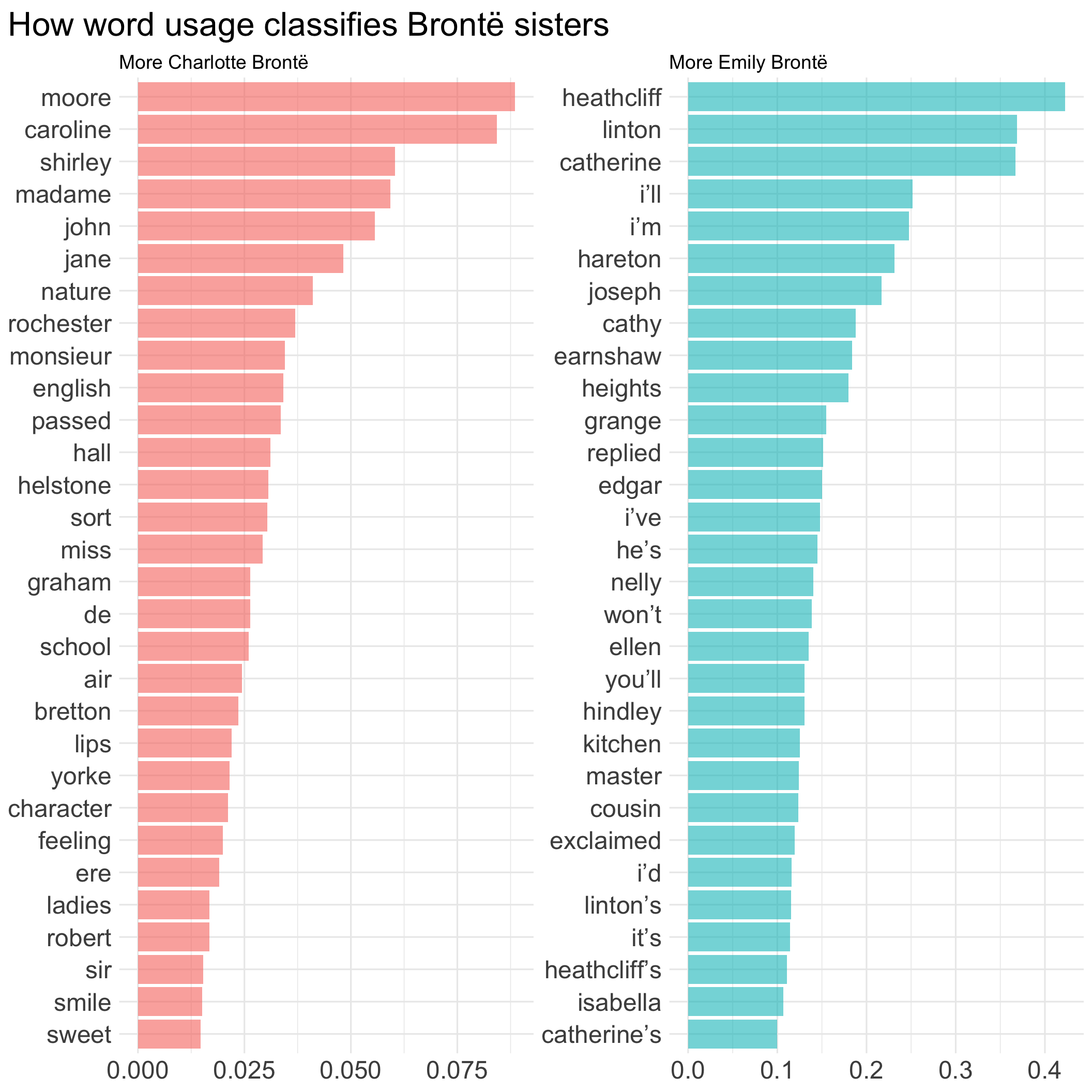
Is it cheating to use names of a character to classify authors? Perhaps I should consider include more books and remove names for text classification next time.
Note that variale importance in the left panel is generally smaller than the right, this corresponds to what we find in the word frequency plot Figure 1 that Emily Brontë has more and stronger characteristic words.